Thermodynamics and Kinetics
Driving Force
The driving force is defined as the maximum difference in Gibbs free energy between the chemical potential hyperplane computed for the matrix ($\alpha$) and precipitate ($\beta$) phase separately. This can also be defined as the difference in the Gibbs free energy when the chemical potential hyperplanes of each phase are parallel. The chemical potential of the $\alpha$ phase is computed at the matrix composition while the chemical potential of the $\beta$ phase is computed at the composition which maximizes the driving force.
$$ \Delta G_{ch} = \sum{x_A^\beta \mu_A^\alpha (\boldsymbol{x^\alpha}) - x_A^\beta \mu_A^\beta (\boldsymbol{x^\beta})} = \left(\frac{2\gamma}{R^*} + \Delta G_{el} \right) V_m^\beta $$
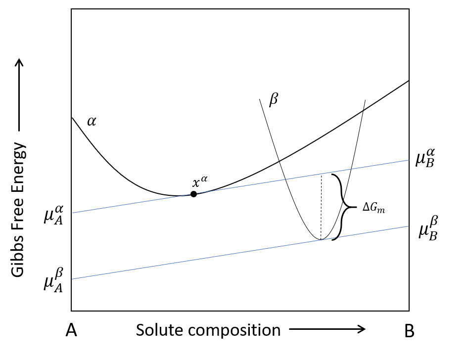
Driving force for a binary system
kawin supports three different methods to calculate the driving force.
Approximate
The approximate method assumes that the composition of a newly nucleated precipitate is near the equilibrium composition. This is the default method when the Thermodynamics object is created.
$$ \Delta G_{ch} = \sum{x_{A,eq}^\beta \mu_A^\alpha (\boldsymbol{x^\alpha}) - x_{A,eq}^\beta \mu_A^\beta (\boldsymbol{x_{eq}^\beta})} $$
Sampling
The sampling method approximates calculating the driving force by the parallel tangent method. Rather than finding the composition of the precipitate phase that gives the same chemical potential as for the parent phase, the maximum difference between Gibbs free energy of the precipitate phase and the chemical potential hyperplane of the parent phase is found. This is the only method of the three that can calculate negative driving forces and is used if the precipitate phase is unstable.
$$ \Delta G_{ch} = max \left(\sum{x_A^\beta \mu_A^\alpha (\boldsymbol{x^\alpha}) - G_m^\beta (\boldsymbol{x^\beta})} \right) $$
Curvature
The curvature method determines the local curvature of the free energy surface of the parent phase at the given composition and calculates driving force based off the equilibrium composition of the parent and precipitate phase. This is only valid for small supersaturations and non-dilute systems and thus, is not recommended.
$$ \Delta G_m = (\boldsymbol{x^\alpha - x_{eq}^\alpha}) \nabla^2 G_m^α (\boldsymbol{x_{eq}^\beta-x_{eq}^\alpha}) $$
Growth Rate
Binary
Assuming diffusion-controlled growth, the growth rate of a spherical precipitate in a binary system can be written as:
$$ \frac{dR}{dt} = \frac{D}{R} \frac{x - x_R^\alpha}{x_R^\beta - x_R^\alpha} $$
Where $x_R^\alpha$ and $x_R^\beta$ is the interfacial composition of the matrix and precipitate phase respectively. For binary systems, the interfacial composition is independent of the composition of the system. This becomes useful in the KWN model as these values can be calculated beforehand and used for determining the growth rate, rather than calculating them at every iteration.
Determining the interfacial composition requires solving for equilibrium while accounting for the Gibbs-Thompson effect (proportional to 1/r). Elastic energy can also be accounted for.
$$ \mu_i^\alpha (x_R^\alpha) = \mu_i^\beta (x_R^\beta) + \left(\frac{2\gamma}{R} + \Delta G_{el} \right) V_m^\beta $$
Multicomponent
The governing equations for solving multicomponent precipitate is the same as for binary precipitation. However, calculating interfacial composition through solving for equilibrium requires the solution to the following equations for each component.
$$ \frac{dR}{dt} = \sum_{j}{\frac{D_{ij}}{R} \frac{x_j - x_{R,j}^\alpha}{x_{R,i}^\beta - x_{R,i}^\alpha}} $$
$$ \mu_i^\alpha (\boldsymbol{x_R^\alpha}) = \mu_i^\beta (\boldsymbol{x_R^\beta}) + \left(\frac{2\gamma}{R} + \Delta G_{el} \right) V_m^\beta $$
This gives 2N-1 equations to solve, which can be time consuming and, in worst cases, a solution may not be found. At small saturations, the growth rate can be determined through local expansion of the chemical potential at equilibrium. The growth rate then becomes:
$$ \frac{dR}{dt} = \frac{1}{R \boldsymbol{(\Delta \overline{x})^T M^{-1} \Delta \overline{x}}} \left(\Delta G_{ch} - \left(\frac{2\gamma}{R} + \Delta G_{el} \right) V_m^\beta \right) $$
$$ \boldsymbol{\Delta \overline{x} = x_\infty^\beta - x_\infty^\alpha} $$
$$ \boldsymbol{M^{-1}} = \nabla^2 G_m^\alpha \boldsymbol{D^{-1}} $$
Where $\boldsymbol{x_\infty^\alpha}$ and $\boldsymbol{x_\infty^\beta}$ are the equilibrium compositions of $\alpha$ and $\beta$ on a planar interface, $ \nabla^2 G_m^\alpha $ is the curvature of the free energy surface of phase $\alpha$ and $ \boldsymbol{D^{-1}} $ is the inverse of the interdiffusivity matrix.
Interfacial compositions can be determined by the following equations, which are useful for solving mass balance. Note that the growth rate calculations are independent of the reference element, where the growth rate will be the same regardless of the chosen reference.
$$ \boldsymbol{x^\alpha} = \boldsymbol{x} - \frac{\boldsymbol{D^{-1} \Delta \overline{x}}}{R \boldsymbol{(\Delta \overline{x})^T M^{-1} \Delta \overline{x}}} \left(\Delta G_{ch} - \left(\frac{2\gamma}{R} + \Delta G_{el} \right) V_m^\beta \right) $$
$$ \boldsymbol{x^\beta} = \boldsymbol{x_\infty^\beta} + \left(\nabla^2 G_m^\beta \right)^{-1} \nabla^2 G_m^\alpha (\boldsymbol{x - x_\infty^\alpha}) $$
References
B. Rheingans and E. Mettemeijer, “Modeling precipitation kinetics: Evaluation of the thermodynamics of nucleation and growth” Calphad: Computer coupling of phase diagrams and thermochemistry 50 (2015) p. 49
Q. Chen, J. Jeppson and J. Agren, “Analytical treatment of diffusion during precipitate growth in multicomponent systems” Acta Materialia 56 (2008) p. 1890
T. Philippe and P. W. Voorhees, “Ostward ripening in multicomponent alloys” Acta Materialia 61 (2013) p. 4237