Kampmann-Wagner Numerical Model
kawin relies on classical nucleation and growth theories to model precipitation behavior in alloys.
There are several ways to model precipitation behavior using these theories. The Langer-Schwartz (LS) model predicts the evolution of the mean radius of particles in near critical fluids. Modification of the LS model (the MLS model) allows it to be applied to supersaturated solid solutions. However, the MLS model only predicts the mean radius, assuming that the particle size distribution follows a Lifshitz-Slyozov-Wagner distribution.
To model the particle size distribution, the Kampmann-Wagner numerical (KWN) model divides the size distribution into size classes that evolves over time. The evolution of these size classes can modeled using a Euler-like approach, where the size classes are fixed and evolution of the size class frequencies are determined by fluxes from neighboring classes. In a Lagrange-like approach, the radius of each size class can grow or shrink while the frequency in each size class is kept constant. Currently, kawin only implements the Euler-like implementation of the KWN model.
Classical nucleation theory (CNT)
The first step in precipitation is nucleation. When a nucleate is formed, the net change in free energy depends on the volume contribution (which decreases the free energy) and surface area contribution (which increases the energy). These two contributions create a nucleation barrier.
$$ \Delta G = -\frac{4}{3} \pi R^3 \Delta G_{v} + 4 \pi R^2 \gamma $$
The volumetric change in free energy, $\Delta G_{v}$ is related to the molar change in free energy or the driving force ($\Delta G_{ch}$) and the elastic strain energy, $\Delta G_{el}$. (Note: the driving force is denoted here such that a positive value means nucleation will lower the volumetric Gibbs free energy).
$$ \Delta G_{v} = \frac{\Delta G_{ch}}{V_m^\beta} + \Delta G_{el} $$
The nucleation barrier occurs at a critical radius ($ R^* $) with a height of $ \Delta G^* $.
$$ R^* = \frac{2 \gamma}{\Delta G_{v}} $$
$$ \Delta G^* = \frac{4}{3} \pi \gamma {R^*}^2 = \frac{16}{3} \frac{\pi \gamma^3}{\Delta G_{v}^2} $$
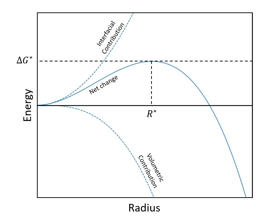
Free energy contributions of a nucleate
In a supersaturated solution, clusters of solute atoms will continually form and decay. Whether these clusters will continue to growth or dissolve depends on the radius of these clusters. Clusters smaller than the critical radius will dissolve while clusters larger than the critical radius are stable and continue to grow. Modeling nucleation behavior only concerns the stable clusters, where the nucleation rate is proportional to the height of the nucleation barrier.
$$ J_{nuc} \propto \exp{\left(-\frac{\Delta G^*}{k_B T}\right)} $$
The nucleation rate depends on several other factors:
- Impingement rate ($\beta$) - the rate at which solute atoms attach to a cluster $$ \beta = \frac{4 \pi {R^*}^2 x_0 D}{a^4} \text{ for binary systems} $$
$$ \beta = \frac{4 \pi {R^*}^2}{a^4} \left(\sum_{i}{\frac{(x_i^\beta - x_i^\alpha)^2}{x_i^\alpha D_i}}\right)^{-1} \text{ for multicomponent systems} $$
Zeldovich factor (Z) - accounts for the probablity that a cluster at the height of the nucleation barrier will continue to grow or decay $$ Z = \frac{V_m^\beta}{2 \pi N_A {R^*}^2} \sqrt{\frac{\gamma}{k_B T}} $$
Nucleation site density ($N_0$) - the number of potential nucleation sites per volume
Incubation time ($\tau$) - characteristic time representing how long it takes for the system to reach steady state where clusters are continually forming and decaying $$ \tau = \frac{1}{2 Z^2 \beta} $$ Note: in other derivations for the incubation time, the 2 may be replaced with $4\pi$.
Using these terms, the nucleation rate can be stated as:
$$ J_{nuc} = N_0 Z \beta \exp{\left(-\frac{\Delta G^*}{k_B T}\right)} \exp{\left(-\frac{\tau}{t}\right)} $$
As precipitates nucleate, they take up nucleation sites. Thus, $N_0$ is subtracted from over time to represent the density of currently available nucleation sites.
Precipitate growth
Assuming the precipitate is spherical and the composition profile is in a quasi-steady state, the composition of the matrix outside the precipitate is the solution to the Laplace equation.
$$ x_i = x_i^\infty + \frac{(x_{R,i}^\alpha - x_i^\infty) R}{r} $$
The interfacial velocity is related to the concentration gradient by
$$ (x_{R,i}^\beta - x_{R,i}^\alpha) \frac{dR}{dt} = \sum_{j}{D_{ij} \frac{dx_j}{dr} \biggr\rvert_{r=R}} $$
Combining these two equations gives the growth rate
$$ \frac{dR}{dt} = \sum_{j}{\frac{D_{ij}}{R} \frac{x_j^\infty - x_j^\alpha}{x_i^\beta - x_i^\alpha}} $$
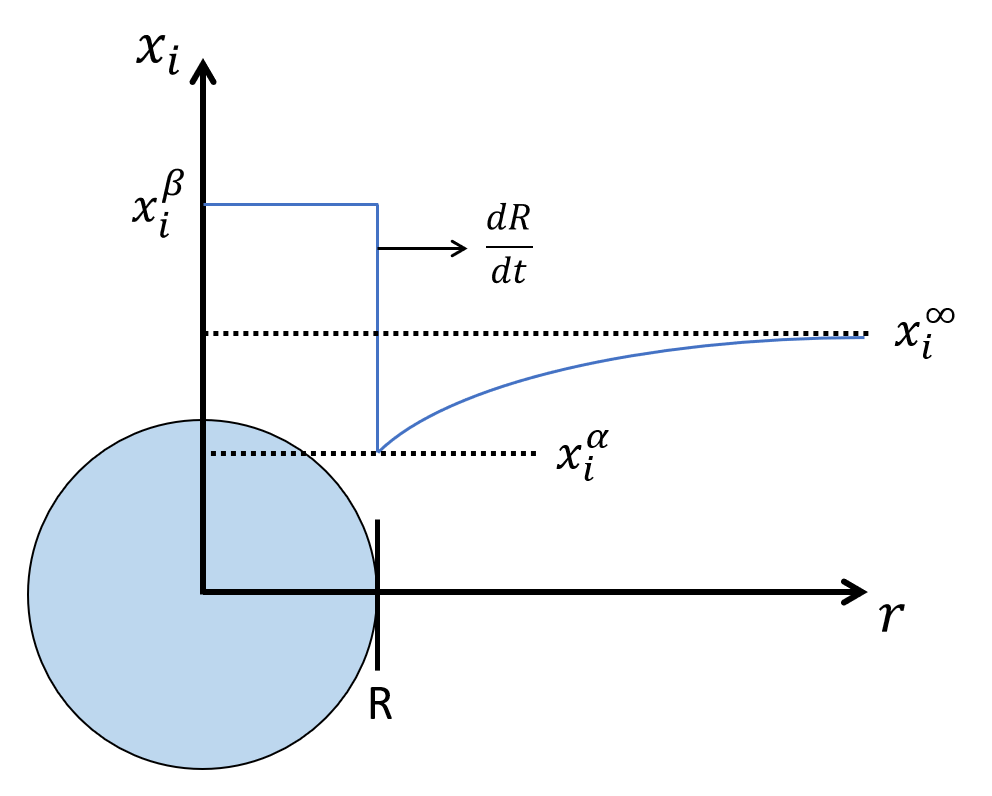
Composition profile from precipitate to matrix phase
Mass Balance
Mass balance is performed by finding the moments of the particle size distribution. The number density, average radius and volume fraction is the zeroth, first and third moment respectively. The volume fraction is unitless since the frequency of each size class is per unit volume.
$$ N_{total} = \sum_{i}{n_i} $$
$$ R_{avg} = \frac{\sum_{i}{n_i R_i}}{\sum_{i}{n_i}} $$
$$ f_v = \frac{4\pi}{3} \sum_{i}{n_i R_i^3} $$
To conserve mass, the sum of solute atoms in the matrix and in the precipitate must be equal to the initial number of solute atoms.
$$ x_{j,0} = (1 - f_v) x_j^\infty + \frac{4\pi}{3} \sum_{i}{n_i R_i^3 x_{R_i,j}^\beta} $$
The above equation assumes infinitely fast diffusion in the precipitate such that the composition of each precipitate is equal to the interfacial composition. The other extreme case would be infinitely slow diffusion, where the composition of the precipitate is dependent on its history. The mass balance equation then becomes
$$ x_{j,0} = (1 - f_v) x_j^\infty + 4\pi \sum_{i}{\sum_{t}{n_{i,t} R_i^2 x_{R_i,j,t}^\beta} \frac{dR}{dt} \biggr\rvert_{i,t} } $$
For nucleation of multiple precipitate phases, the same nucleation and growth theories are used. Coupling is done through the mass balance, where the number of solute atoms are summed over all precipitate phases. For infinitely fast diffusion, the mass balance becomes
$$ x_{j,0} = (1 - \sum_{p}{f_{v,p}}) x_j^\infty + \frac{4\pi}{3} \sum_{p}{\sum_{i}{n_{p,i} R_{p,i}^3 x_{R_{p,i},j}^\beta}} $$
The same can be done for infinitely slow diffusion.
Solving the KWN model
The KWN model is solved through multiple steps. Time constraints are split into two groups: a pre-check and a post-check. The pre-check uses the nucleation and growth rate to determine an optimial time increment while the post-check will check how much the composition and volume changed after an iteration and reduce the time increment if needed.
- Calculate nucleation rate and critical radius
- Calculate growth rate
- Pre-check time constraints
- Update particle size distribution (PSD) with both nucleation and growth rate
- Calculate PSD statistics and update matrix composition
- Post-check time constraints
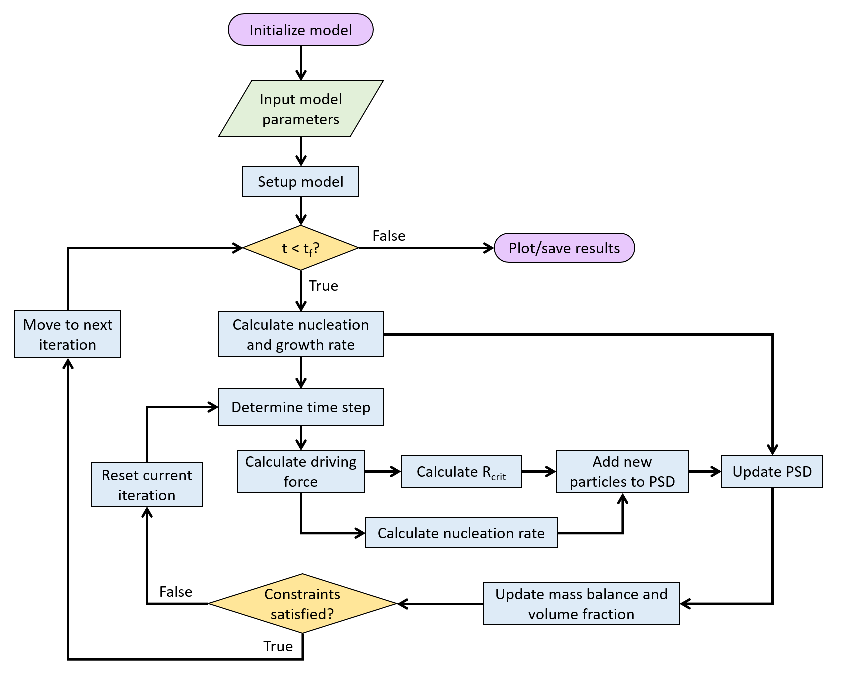
Flowchart for solving the KWN model
References
E. Kozeschnik, Precipitation Modeling. Chapter 2: Precipitate Nucleation, Momentum Press, 2021
M. Perez, M. Dumont and D. Acevedo-Reyes, “Implementation of classical nucleation and growth theories for precipitation” Acta Materialia 56 (2008) p. 2119
Q. Chen, J. Jeppson and J. Agren, “Analytical treatment of diffusion during precipitate growth in multicomponent systems” Acta Materialia 56 (2008) p. 1890