Strain Energy Calculations

Strain energy is produced when there is a difference in molar volume between the precipitate and the matrix. Depending on this difference, work has to be done to compress/stretch the precipitate such that it will fit into the matrix. The work done acts to decrease the driving force for nucleation. For ellipsoidal precipitate shapes, the work done can be calculated by Eshelby’s theory. For spherical and cuboidal shapes, Khachaturyan’s approximation may be used.

Eshelby’s theory #

For ellipsoial precipitates, Eshelby’s theory must be used. The strain energy induced by the precipitate can be viewed as a 4 step process.

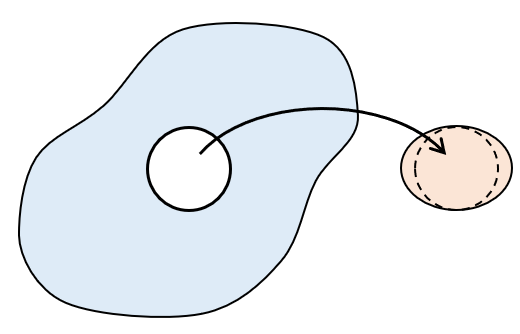
1. Take the inclusion out of the matrix and let it deform to an unstressed state. The total strain on the inclusion will be it’s eigenstrain ($ \varepsilon_{ij}^{*} $).

   

2. Apply traction forces to the inclusion to fit the missing volume in the matrix.

   

   The strain on the precipitate is now zero, but the stress on the precipitate is proportional to it’s eigenstrain (where $C_{ijkl}$ is the elastic tensor of the matrix). $$ \sigma_{ij} = -C_{ijkl} \varepsilon_{ij}^{*} = -\sigma_{ij}^{*} $$ The work done in this step is $$ W_2 = \frac{1}{2} V \sigma_{ij}^{*} \varepsilon_{ij}^{*} $$

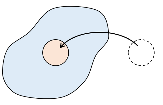
3. Insert the inclusion into the matrix.

   

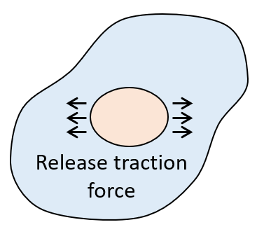
4. Release traction forces and let the inclusion expand into the matrix.

   

   The “constrained” strain induced from this will be denoted as $ \varepsilon_{ij}^{c} $. The stress on the precipitate will then be $$ \sigma_{ij} = C_{ijkl} (\varepsilon_{kl}^{c} - \varepsilon_{kl}^{*}) = \sigma_{ij}^c - \sigma_{ij}^{*} $$ The work done in this step is $$ W_4 = -\frac{1}{2} V \sigma_{ij}^{*} \varepsilon_{ij}^{c} = -\frac{1}{2} V C_{ijkl} \varepsilon_{kl}^{*} \varepsilon_{ij}^{c} = -\frac{1}{2} V \sigma_{ij}^{c} \varepsilon_{ij}^{*} $$

The strain energy induced by the precipitate is determined by the net work done in the 4 steps (work is only done in steps 2 and 4). Thus the net work done is

$$ E = W_2 + W_4 = -\frac{1}{2} V (\sigma_{ij}^{c} - \sigma_{ij}^{*}) \varepsilon_{ij}^{*} $$

The constrained strain is calculated using Eshelby’s tensor ($S_{ijmn}$) which is found from an additional tensor $D_{ijkl}$.

$$ D_{ijkl} = -\frac{abc}{4\pi} \int_{0}^{\pi} \int_{0}^{2\pi} \Omega_{ij} n_k n_l \frac{\sin{\theta}}{\beta^3} d\phi d\theta $$

Where

$$ \beta = \sqrt{(a^2 \cos^2{\phi} + b^2 \sin^2{\phi}) \sin^2{\theta} + c^2 \cos^2{\theta}} $$

$$ \Omega_{ij}^{-1} = C_{ijkl} n_k n_l $$

Eshelby’s tensor can then be calculated by

$$ S_{ijmn} = -\frac{1}{2} C_{lkmn} (D_{iklj} + D_{jkli}) $$

The constrained strain is calculated from Eshelby’s tensor and the eigenstrain, which allows for the elastic strain energy of the precipitate to be found.

$$ \varepsilon_{ij}^c = S_{ijkl} \varepsilon_{kl}^{*} $$

$$ \sigma_{ij}^{*} = C_{ijkl} \varepsilon_{ij}^{*} $$

$$ \sigma_{ij}^{c} = C_{ijkl} \varepsilon_{ij}^{c} $$

$$ E = -\frac{1}{2} (\sigma_{ij}^{c} - \sigma_{ij}^{*}) \varepsilon_{ij}^{*} V $$

Rotation of the elastic tensor #

The previous equations assume that the eigenstrains and elastic tensor are aligned on the same axes. However, this is not always the case. This may occur when the precipitate forms along a certain direction in the unit cell of the matrix phase. Accounting for this requires rotating the elastic tensor using a rotation tensor $r$.

$$ C_{ijkl} = r_{im} r_{jn} r_{ko} r_{lp} C_{mnop} $$

Calculating $D_{ijkl}$ #

$D_{ijkl}$ is solved by numerically integrating over a unit sphere. However, for large aspect ratios, the integrand can vary largely along $\phi$. In kawin, this integral is solved using the Lebedev quadrature. Options are available for using the quadrature of polynomial order 53, 83 and 131 (which represent the highest polynomial order that can be integrated exactly). However, in general, using a polynomial order of 131 is recommended.

Khachaturyan’s Approximation #

For spherical and cuboidal precipitates, the strain energy can be calculated by Khachaturyan’s approximation. The cubic factor, $\eta$, characterizes how close the precipitate is to a perfect sphere or cube. The shape of the precipitate is described by

$$ x^p + y^p + z^p <= R^p $$

$$ \eta = \sqrt{2} * 2^{-1/p} $$

For a sphere, $\eta = 1$, and for a cube, $\eta = \sqrt{2}$.

The elastic energy is then found by

$$ E = \frac{1}{2} (c_{11} + 2c_{12}) \varepsilon_{0}^{2} V (A_1 + A_2) $$

Where $c_{11}$, $c_{12}$ and $c_{44}$ are the elastic constants for cubic systems and

$$ A_1 = 2 \frac{c_{11} - c_{12}}{c_{11}} - 12 \frac{c_{11} + 2c_{12}}{c_{11}} \frac{c_{11} - c_{12} - 2c_{44}}{c_{11} + c_{12} + 2c_{44}} I_1 $$

$$ A_2 = -54 \frac{c_{11} + 2c_{12}}{c_{11}} \frac{(c_{11} - c_{12} - 2c_{44})^2}{(c_{11} + c_{12} + 2c_{44})(c_{11} + 2c_{12} + 4c_{44})} I_2 $$

Where $I_1 = \frac{1}{15}$, $I_2 = \frac{1}{105}$ for a sphere and $I_1 = 0.006931$, $I_2 = 0.000959$ for a cube.

For shapes between a sphere and a cube, the elastic strain energy can be found through linear interpolation with $\eta$. However, kawin does not currently support handling of precipitates with different cubic factors and precipitates are taken to be either a perfect sphere or cube.

Equilibrium Aspect Ratio #

The morphology of a precipitate depends on both the elastic strain energy and the interfacial energy. The aspect ratio is then determined by the minimum of both energy contributions.

$$ \alpha = \text{argmin} \left(\frac{4}{3} \pi R_{sph}^3 E(\alpha) + 4 \pi R_{sph}^2 g(\alpha) \gamma \right) $$

In kawin, this calculation is performed by caching strain energy calculations for a range of aspect ratios (incrementing by 0.01) and searching the aspect ratio that gives the lowest energy contribution. The number of cached calculations will be automatically increased if it’s determined that the equilibrium aspect ratio is larger than the largest cached value.

References #

1. J. D. Eshelby, “The elastic field outside an ellipsoidal inclusion” Proceedings of the Royal Society of London. Series A, Mathematical and Physical Sciences 252 (1959) p. 561

2. C. Weinberger, W. Cai and D. Barneet, ME340B Lecture Notes - Elasticity of Microscopic Structures, Stanford Univerity, 2005. http://micro.stanford.edu/~caiwei/me340b/content/me340b-notes_v01.pdf

3. K. Wu, Q. Chen and P. Mason, “Simulation of precipitation kinetics with non-spherical particles” Journal of Phase Equilibria and Diffusion 39 (2018) p. 571

4. V. I. Lebedev, “Quadratures on a sphere” USSR Computational Mathematics and Mathematical Physics 16 (1976) p. 10