Precipitation with Strain Energy
This example will cover adding a strain energy term to the KWN model. This strain energy term will also be used to calculate the aspect ratio as a function of precipitate radius.
Example - The Cu-Ti system
In copper alloys with dilute amounts of titanium, formation of $\beta$-$Cu_4Ti$, a needle-like precipitate, can occur. Due to volume differences between the precipitate and the parent phase, the parent phase is put under strain. This strain comes with an elastic energy that serves to reduce the driving force for nucleation. In addition, the aspect ratio of the $\beta$ precipitates depends on the size of the precipitate to minimize the elastic and interfacial energy contributions.
To setup the KWN, the PrecipitateModel and BinaryThermodynamics will need to be defined. For BinaryThermodynamics, a mobility correction factor of 100 will be applied. This is to represent the presence of excess quench-in vacancies, which will speed up diffusion.
1  from kawin.thermo import BinaryThermodynamics
2
3  therm = BinaryThermodynamics('CuTi.tdb', ['CU', 'TI'], ['FCC_A1', 'CU4TI'], interfacialCompMethod='equilibrium', drivingForceMethod='approximate')
4  therm.setMobilityCorrection('all', 100)
5  therm.setGuessComposition(0.15)
Model Inputs
For model inputs, the composition will be Cu-1.9Ti (at.%) and the temperature will be $350\text{ }^oC$. The molar volume of the matrix phase will be that of FCC copper with 2 atoms per unit cell. For the $\beta$-$Cu_4Ti$ precipitates, the atomic volume and atoms per unit cell are taken from Ref. 5 from the SpringerMaterials database. Bulk nucleation will be assumed with $1e30\text{ }sites/m^3$.
 6  from kawin.precipitation import MatrixParameters, PrecipitateParameters
 7
 8  matrix = MatrixParameters(['TI'])
 9  matrix.initComposition = 0.019
10  matrix.volume.setVolume(7.11e-6, 'VM', 4)
11  matrix.nucleationSites.setBulkDensity(1e30)
12
13  precipitate = PrecipitateParameters('CU4TI')
14  precipitate.gamma = 0.035
15  precipitate.volume.setVolume(0.25334e-27, 'VA', 20)
16  precipitate.nucleation.setNucleationType('bulk')
Elastic Energy
Elastic energy has to be defined by a separate object, StrainEnergy. Here, the elastic constants and eigenstrains can be defined. It is important to check the order of the axes in the eigenstrains. For needle-like precipitates, the axes are (short axis, short axis, long axis). For plate-like precipitates, the axes are (long axis, long axis, short axis).
When inputting the StrainEnergy object into the KWN model, setting “calculateAspectRatio” to True will allow for the aspect ratio to be calculated from the elastic energy. Otherwise, the aspect ratio will be taken from what was defined when defining the precipitate shape.
17  precipitate.strainEnergy.setElasticConstants(168.4e9, 121.4e9, 75.4e9)
18  precipitate.strainEnergy.setEigenstrain([0.022, 0.022, 0.003])
19  precipitate.calculateAspectRatio = True
20
21  #Set precipitate shape
22  #Since we're calculating the aspect ratio, it does not have to be defined
23  #Otherwise, a constant value or function can be inputted
24  precipitate.shapeFactor.setPrecipitateShape('needle')
Solving the model
25  from kawin.precipitation import PrecipitateModel
26
27  model = PrecipitateModel(matrix, precipitate, therm, 350+273.15)
28  model.solve(1e5, verbose=True, vIt=5000)
N	Time (s)	Sim Time (s)	Temperature (K)	Matrix Comp
0	0.0e+00		0.0		623		1.9000

	Phase	Prec Density (#/m3)	Volume Frac	Avg Radius (m)	Driving Force (J/mol)
	CU4TI	0.000e+00		0.0000		0.0000e+00	1.9660e+03

N	Time (s)	Sim Time (s)	Temperature (K)	Matrix Comp
4127	1.0e+05		65.6		623		0.1758

	Phase	Prec Density (#/m3)	Volume Frac	Avg Radius (m)	Driving Force (J/mol)
	CU4TI	1.476e+23		9.3686		5.0967e-09	1.2302e+02
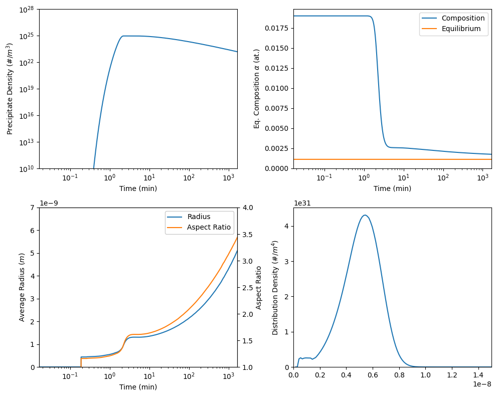
Plotting
As with the other examples, plotting is the same. Some additional things:
- The variable ‘timeUnits’ is set to ‘min’ to plot in minutes rather than seconds
- The equilibrium matrix composition is plotted to compare with the actual composition.
- The mean aspect ratio and aspect ratio as a function of radius is plotted
29  %matplotlib inline
30  import matplotlib.pyplot as plt
31  from kawin.precipitation.Plot import plotPrecipitateResults
32
33  fig, axes = plt.subplots(2, 2, figsize=(10, 8))
34
35  plotPrecipitateResults(model, 'precipitate density', ax=axes[0,0], timeUnits='min')
36  axes[0,0].set_ylim([1e10, 1e28])
37  axes[0,0].set_yscale('log')
38
39  plotPrecipitateResults(model, 'composition', ax=axes[0,1], timeUnits='min', label='Composition')
40  plotPrecipitateResults(model, 'eq comp alpha', ax=axes[0,1], timeUnits='min', label='Equilibrium')
41  axes[0,1].legend()
42
43  plotPrecipitateResults(model, 'average radius', ax=axes[1,0], timeUnits='min', label='Radius', color='C0')
44  axes[1,0].set_ylim([0, 7e-9])
45  ax1 = axes[1,0].twinx()
46  plotPrecipitateResults(model, 'aspect ratio', ax=ax1, timeUnits='min', label='Aspect Ratio', color='C1')
47  ax1.set_ylim([1,4])
48
49  lineR, labelR = axes[1,0].get_legend_handles_labels()
50  lineAR, labelAR = ax1.get_legend_handles_labels()
51  axes[1,0].legend(lineR+lineAR, labelR+labelAR, framealpha=1)
52
53  plotPrecipitateResults(model, 'pdf', ax=axes[1,1])
54  axes[1,1].set_xlim([0, 1.5e-8])
55
56  fig.tight_layout()
References
- A. T. Dinsdale, “SGTE Data for Pure Elements” Calphad 15 (1991) p. 317
- J. Wang et al, “Experimental Investigation and Thermodynamic Assessment of the Cu-Sn-Ti Ternary System” Calphad 35 (2011) p. 82
- J. Wang et al, “Assessment of Atomic Mobilities in FCC Cu-Fe and CuTi Alloys” Journal of Phase Equilibria and Diffusion 32 (2011) p. 30
- K. Wu, Q. Chen and P. Mason, “Simulation of Precipitate Kinetics with Non-Spherical Particles” Journal of Phase Equilibria and Diffusion 39 (2018) p. 571
- Eremenko V.N., Buyanov Y.I., Prima S.B., “Phase diagram of the system titanium-copper” Soviet Powder Metallurgy and Metal Ceramics 5 (1966) p. 494