Single Phase Diffusion
Example - NiCrAl System
Along with precipitation, kawin also supports one dimensional diffusion models. In this example, a diffusion couple will be simulated between two different NiCrAl compositions. Both phases will be FCC.
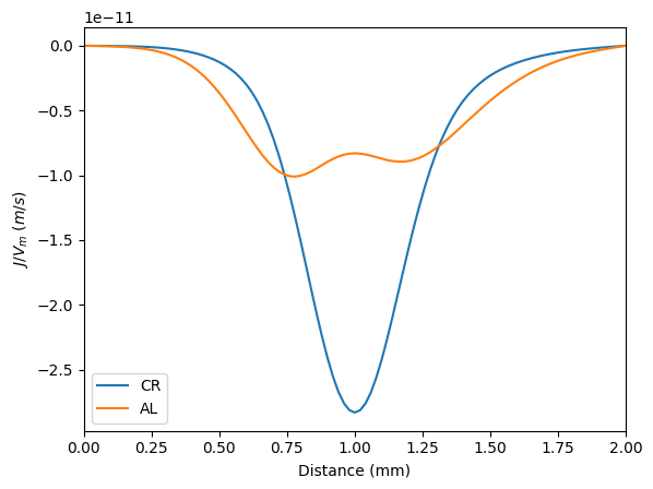
Note: Fluxes are calculated on a volume fixed frame of reference. In this frame of reference, the location of the Matano plane is fixed. If a lattice fixed frame of reference is used, then the movement of the Matano plane would move (this would be similar to the Smigelskas�Kirkendall experiments).
Setup
The diffusion model handles the mesh creation and interfaces with the Thermodynamics module to compute fluxes from mobility and the curvature of the Gibbs free energy surface
Loading the Thermodynamics object is the same as done for creating a precipitation model. The GeneralThermodynamics object can be used here since the functions necessary for the diffusion model are the same for binary and multicomponent systems.
1  from kawin.thermo import GeneralThermodynamics
2
3  therm = GeneralThermodynamics('NiCrAl.tdb', ['NI', 'CR', 'AL'], ['FCC_A1'])
The next step is to create the diffusion model. The model requires the z-coordinates, elements and phases upon initialization. Initial conditions can be added with the composition either as a step function, linear function, delta function or a user-defined function. Finally, boundary conditions are assumed to be no-flux conditions; however, constant flux or composition may also be defined.
Defining the initial and boundary conditions must specify the element it is being applied to.
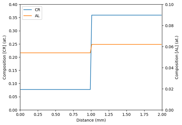
Here, a diffusion couple composed of Ni-7.7Cr-5.4Al / Ni-35.9Cr-6.2Al will be used.
Plotting functions are stored in the diffusion object and can be used to look at the initial conditions.
 4  import matplotlib.pyplot as plt
 5  from kawin.diffusion import SinglePhaseModel
 6  from kawin.diffusion.mesh import ProfileBuilder, StepProfile1D, Cartesian1D
 7  from kawin.diffusion.Plot import plot1DTwoAxis
 8
 9  #Define mesh spanning between -1mm to 1mm with 100 volume elements
10  mesh = Cartesian1D(['CR', 'AL'], [0, 2e-3], 100)
11
12  profile = ProfileBuilder()
13  profile.addBuildStep(StepProfile1D(1e-3, [0.077, 0.054], [0.359, 0.062]), ['CR', 'AL'])
14  mesh.setResponseProfile(profile)
15
16  temperature = 1200+273.15
17  m = SinglePhaseModel(mesh, ['NI', 'CR', 'AL'], ['FCC_A1'],
18                       thermodynamics=therm, temperature=temperature, record=True)
19
20  fig, axL = plt.subplots()
21  axR = axL.twinx()
22  plot1DTwoAxis(m, 'CR', 'AL', zScale=1e-3, axL=axL, axR=axR)
23  axL.set_xlabel('Distance (mm)')
24  axL.set_ylim([0, 0.4])
25  axR.set_ylim([0, 0.1])
Similar to the precipitation model, progress on the simulation can be outputted by setting verbose to True and setting vIt to the number of iterations before a status update on the model is outputted.
26  from kawin.solver import explicitEulerIterator
27  m.solve(100*3600, iterator=explicitEulerIterator, verbose=True, vIt=100)
Iteration	Sim Time (h)	Run time (s)
0		0.0e+00		0.0
100		2.8e+01		4.6
200		5.6e+01		8.8
300		8.4e+01		12.0
356		1.0e+02		13.1
Plotting
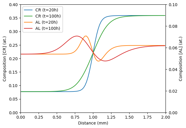
Plotting the final composition profile is the same as plotting the initial profile.
28  fig, axL = plt.subplots()
29  axR = axL.twinx()
30
31  # Plot at 20 hours
32  plot1DTwoAxis(m, 'CR', 'AL', zScale=1e-3, axL=axL, axR=axR,
33                time=20*3600,
34                label={'CR': 'CR (t=20h)', 'AL': 'AL (t=20h)'})
35
36  # Plot at final time
37  plot1DTwoAxis(m, 'CR', 'AL', zScale=1e-3, axL=axL, axR=axR,
38                label={'CR': 'CR (t=100h)', 'AL': 'AL (t=100h)'},
39                color={'CR': 'C2', 'AL': 'C3'})
40  axL.set_xlabel('Distance (mm)')
41  axL.set_ylim([0, 0.4])
42  axR.set_ylim([0, 0.1])
43  from kawin.diffusion.Plot import plot1DFlux
44  fig, ax = plt.subplots()
45  plot1DFlux(m, ['CR', 'AL'], zScale=1e-3, ax=ax)
46  ax.set_xlabel('Distance (mm)')
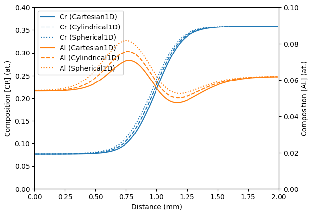
Single phase diffusion in different coordinate systems
The mesh in the single phase diffusion model can be replaced with Cylindrical or Spherical coordinates
47  from kawin.diffusion.mesh import Cylindrical1D, Spherical1D
48  meshes = [
49      Cartesian1D(['CR', 'AL'], [0, 2e-3], 100),
50      Cylindrical1D(['CR', 'AL'], [0, 2e-3], 100),
51      Spherical1D(['CR', 'AL'], [0, 2e-3], 100)
52  ]
53  linestyles = ['-', '--', ':']
54  labels = ['cartesian', 'cylindrical', 'spherical']
55  fig, axL = plt.subplots()
56  axR = axL.twinx()
57  for i, mesh in enumerate(meshes):
58      mesh.setResponseProfile(profile)
59      m = SinglePhaseModel(mesh, ['NI', 'CR', 'AL'], ['FCC_A1'], therm, temperature, record=False)
60      m.solve(100*3600, iterator=explicitEulerIterator, verbose=True, vIt=300)
61
62      plot1DTwoAxis(m, 'CR', 'AL', zScale=1e-3, axL=axL, axR=axR, linestyle=linestyles[i],
63                    label={'AL': f'Al ({mesh.__class__.__name__})', 'CR': f'Cr ({mesh.__class__.__name__})'})
64
65  axL.set_xlabel('Distance (mm)')
66  axL.set_ylim([0, 0.4])
67  axR.set_ylim([0, 0.1])
Iteration	Sim Time (h)	Run time (s)
0		0.0e+00		0.0
300		8.4e+01		12.9
356		1.0e+02		14.3
Iteration	Sim Time (h)	Run time (s)
0		0.0e+00		0.0
300		8.4e+01		22.2
357		1.0e+02		27.3
Iteration	Sim Time (h)	Run time (s)
0		0.0e+00		0.0
300		8.4e+01		22.3
357		1.0e+02		27.2
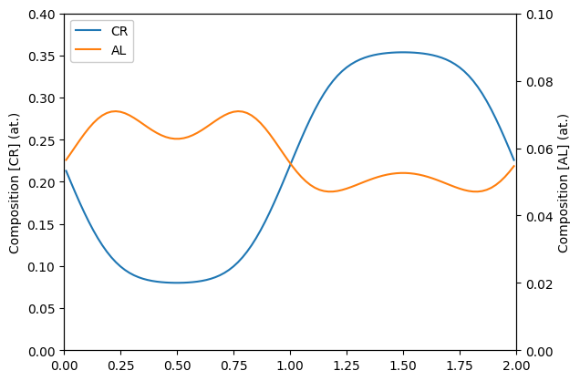
Periodic boundary conditions
68  from kawin.diffusion.mesh import PeriodicBoundary1D
69
70  mesh = Cartesian1D(['CR', 'AL'], [0, 2e-3], 100)
71  mesh.setResponseProfile(profile, boundaryConditions=PeriodicBoundary1D())
72  m = SinglePhaseModel(mesh, ['NI', 'CR', 'AL'], ['FCC_A1'], therm, temperature, record=False)
73  m.solve(100*3600, iterator=explicitEulerIterator, verbose=True, vIt=100)
74
75  fig, axL = plt.subplots()
76  axR = axL.twinx()
77  plot1DTwoAxis(m, 'CR', 'AL', zScale=1e-3, axL=axL, axR=axR)
78  axL.set_ylim([0, 0.4])
79  axR.set_ylim([0, 0.1])
Iteration	Sim Time (h)	Run time (s)
0		0.0e+00		0.0
100		2.8e+01		4.5
200		5.7e+01		9.0
300		8.9e+01		16.1
331		1.0e+02		18.9
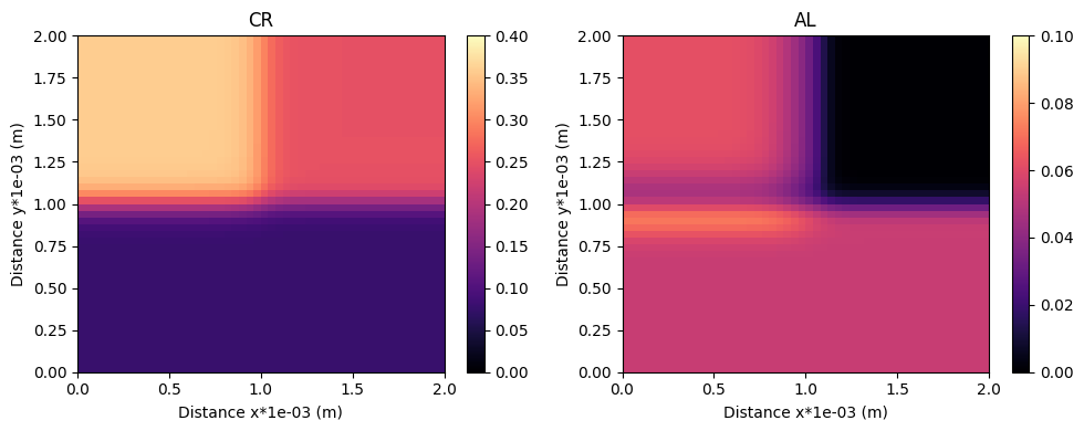
2D mesh
80  from kawin.diffusion.mesh import Cartesian2D, BoundedRectangleProfile
81  from kawin.diffusion.Plot import plot2D
82
83  mesh = Cartesian2D(['CR', 'AL'], [0, 2e-3], 50, [0, 2e-3], 50)
84  profile2d = ProfileBuilder()
85  profile2d.addBuildStep(BoundedRectangleProfile([0,0], [2e-3, 1e-3], [0.077, 0.054]), ['CR', 'AL'])
86  profile2d.addBuildStep(BoundedRectangleProfile([0,1e-3], [1e-3, 2e-3], [0.359, 0.062]), ['CR', 'AL'])
87  profile2d.addBuildStep(BoundedRectangleProfile([1e-3,1e-3], [2e-3,2e-3], [0.25, 0.0]), ['CR', 'AL'])
88  mesh.setResponseProfile(profile2d)
89
90  m = SinglePhaseModel(mesh, ['NI', 'CR', 'AL'], ['FCC_A1'], therm, temperature, record=False)
91  m.solve(20*3600, iterator=explicitEulerIterator, verbose=True, vIt=10)
92
93  fig, ax = plt.subplots(1,2,figsize=(10,4))
94  _, cm = plot2D(m, 'CR', zScale=1e-3, ax=ax[0], cmap='magma', vmin=0, vmax=0.4)
95  fig.colorbar(cm, ax=ax[0])
96  _, cm = plot2D(m, 'AL', zScale=1e-3, ax=ax[1], cmap='magma', vmin=0, vmax=0.1)
97  fig.colorbar(cm, ax=ax[1])
98  fig.tight_layout()
Iteration	Sim Time (h)	Run time (s)
0		0.0e+00		0.0
10		5.6e+00		1.5
20		1.1e+01		5.2
30		1.7e+01		10.6
36		2.0e+01		14.6
References
- A. Borgenstam, A. Engstrom, L. Hoglund, J. Agren, “DICTRA, a Tool for Simulation of Diffusional Transformations in Alloys” Journal of Phase Equilibria 21 (2000) p. 269
- A. Engstrom and J. Agren, “Assessment of Diffusional Mobilities in Face-Centered Cubic Ni-Cr-Al Alloys” Z. Metallkd. 87 (1996) p. 92