Binary Precipitation
Example - The Al-Zr system
In the Al-Zr system, $Al_3Zr$ can precipitate into an $\alpha$-Al (FCC) matrix. The Thermodynamics module provides some functions to interface with pyCalphad in defining the driving force and interfacial composition. However, it is also possible to use user-defined functions for the driving force and nucleation as long as the function parameters and return values are consistent with the ones provides by the Thermodynamics module. Calphad models for the Al-Zr system was obtained from the STGE database and Wang et al [1,2].
For a binary system, one hyperparameter that may need to be set in the Thermodynamics module for calculating interfacial compositions is the guess composition when finding a tie-line. The $Al_3Zr$ phase has a fixed composition at 25 at.% Zr, so the guess composition can be set to 24 at.% Zr.
Since the tdb file does not define diffusivities, we’ll have to define them manually. The diffusivity of Zr in Al-Zr is below [3]. $$ D = 0.0768 , exp\left(- \frac{242000}{R T}\right) : m^2/s $$
 1  import numpy as np
 2  from kawin.thermo import BinaryThermodynamics
 3
 4  therm = BinaryThermodynamics('AlScZr.tdb', elements=['AL', 'ZR'], phases=['FCC_A1', 'AL3ZR'])
 5  therm.setGuessComposition(0.24)
 6
 7  D0 = 0.0768         #Diffusivity pre-factor (m2/s)
 8  Q = 242000          #Activation energy (J/mol)
 9  diff = lambda T: D0 * np.exp(-Q / (8.314 * T))
10  therm.setDiffusivity(diff, 'FCC_A1')
Setting up the model
The KWN model is set up by parameters corresponding to the matrix and precipitate phases. The interfacial energy is taken from Robson and Prangnell [3].
$ x_0 = 0.4 : \text{at.%} $
$ T = 450 : \degree C = 723.15 : K $
$ \gamma = 0.1 : J/m^2 $
$ a = 0.405 : nm = 0.405\mathrm{e}{-9} : m $
4 atoms per unit cell
Dislocation density $ \rho_D = 1e15 /m^2 $
When we set up the matrix parameters, we have to define the solutes. For the precipitate parameters, we need to define the phase name.
11  from kawin.precipitation import MatrixParameters, PrecipitateParameters
12
13  a = 0.405e-9      # nm
14  Va = a**3         # nm^3
15  atomsPerCell = 4
16
17  matrix = MatrixParameters(solutes=['ZR'])
18  matrix.initComposition = 4e-3   # Mole fraction
19  matrix.volume.setVolume(Va, 'VA', atomsPerCell)
20  matrix.nucleationSites.setDislocationDensity(1e15)
21
22  precipitate = PrecipitateParameters('AL3ZR')
23  precipitate.gamma = 0.1   # J/m2
24  precipitate.volume.setVolume(Va, 'VA', atomsPerCell)
25  precipitate.nucleation.setNucleationType('dislocations')
26
27  temperature = 723.15   # Temperature in Kelvin
Solving the Model
Now we can run the model. The current status of the model may be output by setting “verbose” to True with “vIt” being how many iterations will pass before the current status of the model is printed out.
28  from kawin.precipitation import PrecipitateModel
29
30  model = PrecipitateModel(matrix, precipitate, thermodynamics=therm, temperature=temperature)
31  model.solve(500*3600, verbose=True, vIt=10000)
N	Time (s)	Sim Time (s)	Temperature (K)	Matrix Comp
0	0.0e+00		0.0		723		0.4000

	Phase	Prec Density (#/m3)	Volume Frac	Avg Radius (m)	Driving Force (J/mol)
	AL3ZR	0.000e+00		0.0000		0.0000e+00	5.7737e+03

N	Time (s)	Sim Time (s)	Temperature (K)	Matrix Comp
3568	1.8e+06		30.4		723		0.0126

	Phase	Prec Density (#/m3)	Volume Frac	Avg Radius (m)	Driving Force (J/mol)
	AL3ZR	1.374e+22		1.5504		6.1126e-09	3.2843e+02
Plotting
We can now plot the results. Here, we are plotting the precipitate density, volume fraction and average radius as a function of time and the size distribution density at the final time.
Everything will be plotted on a logarithmic time scale.
32  %matplotlib inline
33  import matplotlib.pyplot as plt
34  from kawin.precipitation.Plot import plotPrecipitateResults
35
36  fig, axes = plt.subplots(2, 2, figsize=(10, 8))
37
38  plotPrecipitateResults(model, 'precipitate density', ax=axes[0,0])
39  plotPrecipitateResults(model, 'volume fraction', ax=axes[0,1])
40  plotPrecipitateResults(model, 'average radius', ax=axes[1,0], label=r'$R_{avg}$')
41  plotPrecipitateResults(model, 'critical radius', ax=axes[1,0], label=r'$R_{crit}$')
42  axes[1,0].legend()
43  plotPrecipitateResults(model, 'pdf', ax=axes[1,1])
44
45  fig.tight_layout()
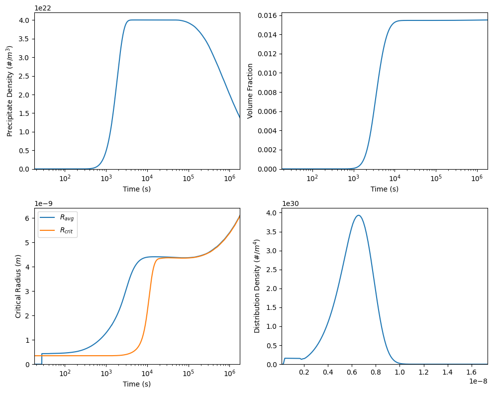
plotPrecipitateResults, where the options are:
- ‘volume fraction’
- ‘critical radius’
- ‘average radius’
- ‘volume average radius’ - average radius given volume fraction
- ‘aspect ratio’ - average aspect ratio
- ‘driving force’
- ‘nucleation rate’
- ‘precipitate density’
- ‘temperature’
- ‘composition’
- ‘eq comp alpha’ - equilibrium composition of matrix phase
- ‘eq comp beta’ - equilibrium composition of precipitate phase
- ‘supersaturation’
- ‘eq volume fraction’ - equilibrium volume fraction of precipitate phase
- ‘psd’ - particle size distribution
- ‘pdf’ - particle size distribution density
- ‘cdf’ - particle cumulative size distribution
The plotPrecipitateResults is a wrapper calling the term-specific plot functions. You can use these function as an alternative as well.
- plotVolumeFraction
- plotCriticalRadius
- plotAverageRadius
- plotVolumeAverageRadius
- plotAspectRatio
- plotDrivingForce
- plotNucleationRate
- plotPrecipitateDensity
- plotTemperature
- plotComposition
- plotEqMatrixComposition
- plotEqPrecipitateComposition
- plotSupersaturation
- plotEqVolumeFraction
- plotSizeDistribution
- plotDistributionDensity
- plotCumulatieDistribution
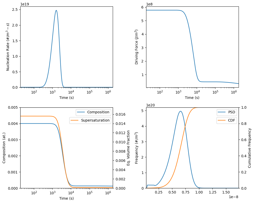
46  import matplotlib.pyplot as plt
47  from kawin.precipitation.Plot import plotNucleationRate, plotDrivingForce, plotComposition, plotSupersaturation, plotSizeDistribution, plotCumulativeDistribution
48
49  fig, axes = plt.subplots(2, 2, figsize=(10, 8))
50
51  plotNucleationRate(model, ax=axes[0,0])
52  plotDrivingForce(model, ax=axes[0,1])
53
54  plotComposition(model, ax=axes[1,0], color='C0', label='Composition')
55  axes[1,0].set_ylim([0, 0.005])
56  ax10Twin = axes[1,0].twinx()
57  plotSupersaturation(model, ax=ax10Twin, color='C1', label='Supersaturation')
58  ax10Twin.set_ylim([0, 0.0175])
59  axes[1,0].legend(loc='upper right')
60  ax10Twin.legend(loc='upper right', bbox_to_anchor=[1, 0.9])
61
62  plotSizeDistribution(model, ax=axes[1,1], color='C0', label='PSD')
63  ax11Twin = axes[1,1].twinx()
64  plotCumulativeDistribution(model, ax=ax11Twin, color='C1', label='CDF')
65  axes[1,1].legend(loc='upper right')
66  ax11Twin.legend(loc='upper right', bbox_to_anchor=[1, 0.9])
67
68  fig.tight_layout()
Saving
The data in the model can be saved into a numpy .npz format
PrecipitateModel.save(filename)
Since only the data is saved, to load the data back in, the model is to be initialized, then the data can be loaded into the model
model = PrecipitateModel(...)
model.load(filename)
References
- A. T. Dinsdale, “SGTE Data for Pure Elements” Calphad 15 (1991) p. 317
- T. Wang, Z. Jin and J. Zhao, �Thermodynamic Assessment of the Al-Zr Binary System� Journal of Phase Equilibria 22 (2001) p. 544
- J. D. Robson and P. B. Prangnell, �Dispersoid Precipitation and Process Modeling in Zirconium Containing Commercial Aluminum Alloys� Acta Materialia 49 (2001) p. 599